Estimating Vehicle Ego-Motion and Piecewise Planar Scene Structure from Optical Flow in a Continuous Framework

GCPR 2015 slides

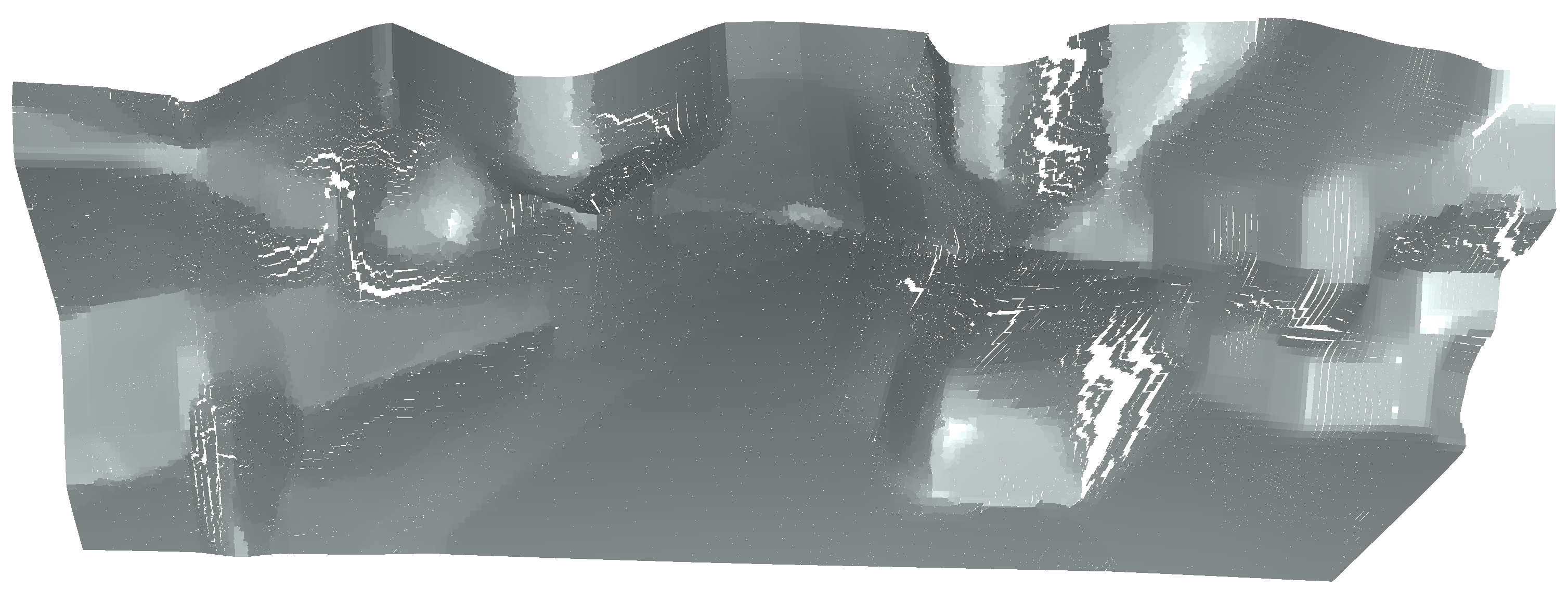
We estimate a 3D scene structure and the vehicle egomotion given the forward and backward optical flow fields between two consecutive frames.

$$ \Downarrow $$

The frames are decomposed into superpixels using the SLIC algorithm, a 3D plane is estimated for each superpixel. Together with the vehicle egomotion, an optical flow field is induced, which is compared to the measured flow. Our method does not utilize a calibrated stereo setup.

Approach

We briefly explain our parametrization and energy formulation on the webpage, see the paper for a detailed explanation. A plane is given by a normal vector $n$ on the sphere $S(2)$, and distance $d \in \mathbb{R}$ from the origin. The plane equation reads $$ n^\top x = d \quad \Leftrightarrow \quad v^\top x = 1, ~ v = \frac{n}{d} $$

Given rotation $R \in \text{SO}(3)$, translation $t \in S(2)$ and 3D point $X$, the point $X'$ relative to the second camera is given by $X' = R^\top (X - t)$. The translation is restricted to the unit sphere, since the translation norm cannot be estimated without additional information. Let $\pi$ denote the projection onto the image plane, $$ \pi\begin{pmatrix} x_1 \\ x_2 \\ x_3 \end{pmatrix} = \frac{1}{x_3} \begin{pmatrix} x_1 \\ x_2 \\ x_3 \end{pmatrix}. $$ Let $z(x)$ denote the depth of pixel $x$ in the image plane, $X = z(x) x$. Depth can be calculated from the plane parameters, $z(x,v) = (v^\top x)^{-1}$. Optical flow is given by $$\begin{align} u(x;R,t,v) = x'(R,t,v) - x &= \pi(R^\top (z(x) x - t)) - x \\ &= \pi (R^\top (x - \frac{t}{z(x)})) - x \\ &= \pi(R^\top (I - t v^\top) x) - x. \end{align}$$ Optical flow is defined by $R$, $t$ and $v$ as shown above, hence we can define an energy function in terms of optical flow, to which we add other energy function for piecewise planar regularity. The energy is minimized using the Levenberg-Marquardt algorithm, respecting the manifold constraints.

Variational Method

Our energy function $E(R,t,v)$ decomposes into $$E(R,t,v) = E_u(R,t,v) + \lambda_z E_z(v) + \lambda_v E_v (v) + \lambda_p E_p (v) \label{eq:energyFunctionComponents},$$ where $E_u$ is the data fidelity term, $E_z$ and $E_v$ are priors on the depth and the plane parameters, respectively and $E_p$ is a term penalizing negative depth values.

The data fidelity term is given by the squared difference between parametrized and estimated optical flow $\hat u(x)$, $$E_u(R,t,v) := \sum_{i=1}^n\! \sum_{x \in \Omega^i} \! w_{\hat{u}}(x) \lVert u(x;R,t,v^i) - \hat u(x) \rVert_2^2.$$ The weights are computed from the forward and backward optical flow between the two input images.

In order to encourage sharp edges in the scene, we choose the robust generalized Charbonnier functional $\rho_C(x) = (x^2+\epsilon)^\alpha - \epsilon^\alpha$, with $\alpha = 1/4$ and $\epsilon = 10^{-10}$. The set $\mathcal{N}_\Omega$ contains all neighboring superpixel pairs.

The first regularity term $E_z(v)$ penalizes depth discontinuities between neighboring superpixels, $$E_z(v) := \sum_{(i,j) \in \mathcal{N}_\Omega} \sum_{x\in \partial^{ij}} w_\Omega^{ij} \rho_C^2 ( x^\top v^i - x^\top v^j ),$$ where $\partial^{ij}$ denotes the boundary between superpixels $i$ and $j$. The weights $w_\Omega^{ij}$ are based on the pixel grey values.

In addition to depth discontinuities, we penalize changes of plane parameters between superpixels, in order to encourage large planar regions, $$E_v(v) = \sum_{(i,j) \in \mathcal{N}_\Omega} w_\Omega^{ij} \| \rho_C( v^i - v^j ) \|_2^2.$$

As additional constraint, we require psoitive depth maps. This is achieved through a soft hinge loss function on the inverse depth at the superpixel center points, $$E_p(v) = \sum_{i=1}^n \rho_+^2( z^{-1}(x_c^i,v^i) ), \quad\text{with}\quad \rho_+(x) := \begin{cases} 1-2x & x \leq 0 \\ (1-x)^2 & 0 < x \leq 1 \\ 0 & 1 < x \end{cases}$$

Optimization

The proposed energy function is non-convex in rotation $R \in \text{SO}(3)$, $t \in S(2)$ and planes $v_i \in \mathbb{R}^3$. We choose the Levenberg-Marquardt algorithm for optimization. Note that the energy can be written in form $$E(R,t,v) = \sum_j \left( f_j(R,t,v) \right)^2 = \lVert f(R,t,v) \rVert_2^2,$$ which can be optimized using Levenberg-Marquardt. We apply a damping factor, which is updated after each iteration.

Results

We demonstrate the output of our algorithms on a few examples here, the paper contains a quantitative evaluation. From top to bottom, each example shows the reference frame, estimated depth and normals and the flow error as measured in the paper (click for a full size view). Depth and depth error (in pixels) are encoded as follows, the scale is derived from ground truth data.

The normal is color-encoded based on the approximately equidistant LAB colorspace. The next image shows the encoding after applying the Hammer-Aitov projection to a sphere and a simple ray-traced scene.

References

- Neufeld, A.; Berger, J.; Becker, F.; Lenzen, F. and Schnörr, C. Estimating Vehicle Ego-Motion and Piecewise Planar Scene Structure from Optical Flow in a Continuous Framework. In 37th German Conference on Pattern Recognition, 2015. pdf BibTeX